更高效的支持向量机算法实现及其在手写数字识别中的应用——01调库实现SVM手写数字识别

大数据机器学习课程第二次实验项目

本文是更高效的支持向量机算法实现及其在手写数字识别中的应用系列文章第01篇——调库实现SVM手写数字识别。

上文我们已经了解了数据的加载与预处理，并且理解了理论上的一些问题。

dataset_dict_uci_digits = load_digits(as_frame=False)
X_train, X_val, X_test, y_train, y_val, y_test, train_set, val_set, test_set, data_module, categories = process_sklearn_dataset_dict(dataset_dict_uci_digits, 'all')
dataset_dict_full_mnist = fetch_openml("mnist_784", as_frame=True)
X_train_full, X_val_full, X_test_full, y_train_full, y_val_full, y_test_full, train_set_full, val_set_full, test_set_full, data_module_full, categories_full = process_sklearn_dataset_dict(dataset_dict_full_mnist, 'all')

(1797, 64) float32 (1797,) int64 [0 1 2 3 4 5 6 7 8 9]
1293 144 360
(70000, 784) float32 (70000,) int64 [0 1 2 3 4 5 6 7 8 9]
50400 5600 14000

1 实验内容

1.1 调库实现SVM

为了给我们后面的实验一个参照，我们调用现有代码库的SVM，关注其精度与速度的情况。 当然如果我们Project在此收尾，只能酌情被扣除分数。 在本节之后，我们将使用 PyTorch 和 numpy 这样的基础科学计算库，来在GPU和CPU上实现SVM及其优化。

!!! important

本次Project首先展示了几个常用的SVM库的精度与速度，并且对其进行调参；随后本次Project基于基础科学计算库手写实现了SVM及其优化，和前面的库的精度与速度进行了对比。

1.1.1 sklearn实现的 SMO 形式的 RBF kernel SVM

from sklearn.svm import SVC

svc = SVC(kernel='rbf', probability=True)
svc.fit(X_train, y_train)

SVC(probability=True)

In a Jupyter environment, please rerun this cell to show the HTML representation or trust the notebook.
On GitHub, the HTML representation is unable to render, please try loading this page with nbviewer.org.

y_pred = svc.predict(X_test)
y_pred_proba = svc.predict_proba(X_test)
svc_res = compute_classification_metrics(y_test, y_pred_proba, logits_to_prob=False, y_pred=y_pred, labels=list(range(10)))
svc_res

{
    'acc1': 0.9722222222222222,
    'acc2': 0.9833333333333333,
    'acc3': 0.9916666666666667,
    'acc5': 0.9916666666666667,
    'acc10': 1.0,
    'acc20': 1.0,
    'matthews_corrcoef': 0.9692503039897137,
    'f1': 0.972029880729665,
    'precision': 0.973182392919235,
    'recall': 0.971984126984127,
    'balanced_accuracy': 0.971984126984127,
    'cohen_kappa': 0.9691339500827382,
    'roc_auc': 0.9993403631348077,
    'hinge_loss': 0.11966705184959518,
    'log_loss': 0.1287164515187897,
    'acc1_pred': 0.9722222222222222
}

需要注意的是，SVM的概率计算的机制较为特殊，所以用SVM的概率预测值进行决策的话，与SVM本身的预测是有所不同的。 因此我们上面看到的结果中，根据y_pred_proba计算的acc1(top k 准确率) 与 根据 y_pred计算的acc1并不相同，SVM本身的预测比SVM的概率预测更加准确。

我写的代码库 namable_classify 就充分考虑了这种情况的发生，允许用户传入 y_pred。

为了更好理解，我们代码可以看到具体的区别在哪里：

import numpy as np

interested = np.where(np.argmax(y_pred_proba, axis=1)!=y_pred)
y_pred_proba[interested], np.argmax(y_pred_proba, axis=1)[interested], y_pred[interested]

(
    array([[0.04655995, 0.06806033, 0.01481866, 0.01379496, 0.04681734,
        0.08531872, 0.31274431, 0.02019028, 0.37692727, 0.01476818],
       [0.00642917, 0.04689452, 0.01313312, 0.04944728, 0.01523242,
        0.03770956, 0.00456987, 0.3768156 , 0.01336737, 0.43640109],
       [0.13989772, 0.01654543, 0.16119182, 0.17785276, 0.05271123,
        0.13162163, 0.13944642, 0.02354677, 0.03741341, 0.1197728 ]]),
    array([8, 9, 3]),
    array([6, 7, 2])
)

1.1.2 sklearn 实现的 SMO形式 的 linear SVM

svc_linear = SVC(kernel='linear', probability=True)
svc_linear.fit(X_train, y_train)

SVC(kernel='linear', probability=True)

In a Jupyter environment, please rerun this cell to show the HTML representation or trust the notebook.
On GitHub, the HTML representation is unable to render, please try loading this page with nbviewer.org.

y_pred = svc_linear.predict(X_test)
y_pred_proba = svc_linear.predict_proba(X_test)
compute_classification_metrics(y_test, y_pred_proba, logits_to_prob=False, y_pred=y_pred, labels=list(range(10)))

{
    'acc1': 0.9777777777777777,
    'acc2': 1.0,
    'acc3': 1.0,
    'acc5': 1.0,
    'acc10': 1.0,
    'acc20': 1.0,
    'matthews_corrcoef': 0.9723041620958817,
    'f1': 0.9748756231876998,
    'precision': 0.9756801209103841,
    'recall': 0.9748326898326898,
    'balanced_accuracy': 0.9748326898326898,
    'cohen_kappa': 0.9722207932506817,
    'roc_auc': 0.9995142149923252,
    'hinge_loss': 0.13536783910745212,
    'log_loss': 0.1218441979874856,
    'acc1_pred': 0.975
}

1.1.3 sklearn 实现的 基于 liblinear 库 的 Linear SVM

The main differences between LinearSVC and SVC lie in the loss function used by default, and in the handling of intercept regularization between those two implementations.

n_samples, n_features = X_train.shape
sklearn_will_use_dual_problem = n_samples < n_features
n_samples, n_features, sklearn_will_use_dual_problem

(1293, 64, False)

from sklearn.svm import LinearSVC

linear_svc = LinearSVC(penalty='l2', loss='squared_hinge', dual=sklearn_will_use_dual_problem, 
                       tol=0.0001, C=1.0, multi_class='ovr', fit_intercept=True, intercept_scaling=1)
linear_svc.fit(X_train, y_train)

LinearSVC(dual=False)

In a Jupyter environment, please rerun this cell to show the HTML representation or trust the notebook.
On GitHub, the HTML representation is unable to render, please try loading this page with nbviewer.org.

y_pred = linear_svc.predict(X_test)
compute_classification_metrics(y_test, y_pred=y_pred, labels=list(range(10)), y_pred_metrics_only=True)

{
    'matthews_corrcoef': 0.9507782171913305,
    'f1': 0.9551493507947526,
    'precision': 0.9564648995608748,
    'recall': 0.9553131703131704,
    'balanced_accuracy': 0.9553131703131704,
    'cohen_kappa': 0.9506151669738929,
    'acc1_pred': 0.9555555555555556
}

1.1.4 sklearn 实现的 SGD优化Hinge Loss形式 的 linear SVM

https://scikit-learn.org/1.5/modules/generated/sklearn.linear_model.SGDClassifier.html

sklearn实现的 soft-margin linear Support Vector Machine 在 from sklearn.linear_model import SGDClassifier类中给出。 sklearn使用的是 one versus all (OVA) scheme，文档摘录如下

For each of the classes, a binary classifier is learned that discriminates between that and all other classes. At testing time, we compute the confidence score (i.e. the signed distances to the hyperplane) for each classifier and choose the class with the highest confidence.

sklearn文档指出这种形式的SVM的潜在优化，包括以下几点

• modified_huber，这是一个平滑版本的hinge loss，有研究表明效果更好。
• ASGD，这个似乎类似于深度学习中的 Stochastic Weight Averaging (SWA)、Model Exponential moving average (Model EMA)和Sharpness-Aware Minimization (SAM)，我们有空深入研究一下这里面的区别与联系。
• Elastic Net, 结合了L1和L2的正则项，来控制模型复杂度。
• optimal learning rate, 具体来说是 Leon Bottou 提出的一种方法，公式在此处可见。

from sklearn.linear_model import SGDClassifier

sgd_svm = SGDClassifier(
    # loss="hinge", 
# penalty="l2", 
    loss="modified_huber", 
                    penalty="elasticnet", 
                    max_iter=1000, fit_intercept=True, 
                    learning_rate='optimal', 
                    early_stopping=True, validation_fraction=0.1, n_iter_no_change=5, warm_start=True, average=True)
sgd_svm.fit(X_train, y_train)

SGDClassifier(average=True, early_stopping=True, loss='modified_huber',
              penalty='elasticnet', warm_start=True)

In a Jupyter environment, please rerun this cell to show the HTML representation or trust the notebook.
On GitHub, the HTML representation is unable to render, please try loading this page with nbviewer.org.

y_pred = sgd_svm.predict(X_test)
compute_classification_metrics(y_test, y_pred=y_pred, labels=list(range(10)), y_pred_metrics_only=True)

{
    'matthews_corrcoef': 0.9538068512149889,
    'f1': 0.9581518233244193,
    'precision': 0.9591395565079776,
    'recall': 0.958086658086658,
    'balanced_accuracy': 0.958086658086658,
    'cohen_kappa': 0.9537005281569381,
    'acc1_pred': 0.9583333333333334
}

1.1.5 使用更加高性能的SVM库来加速训练

1.1.5.1 CPU上对SVM训练的加速

我们首先尝试CPU上的加速。针对英特尔CPU，Intel对sklearn库进行了加速，我们通过下面的方式启用

pip install scikit-learn-intelex

参考 博客 进行测速。

# 加速之前
original_sklearn = [0]*4
original_sklearn[0] = %timeit -o svc.fit(X_train, y_train)
original_sklearn[1] = %timeit -o  svc_linear.fit(X_train, y_train)
original_sklearn[2] = %timeit -o linear_svc.fit(X_train, y_train)
original_sklearn[3] = %timeit -o sgd_svm.fit(X_train, y_train)

235 ms ± 39.9 ms per loop (mean ± std. dev. of 7 runs, 1 loop each)
94.6 ms ± 6.33 ms per loop (mean ± std. dev. of 7 runs, 10 loops each)
232 ms ± 16.9 ms per loop (mean ± std. dev. of 7 runs, 1 loop each)
79.5 ms ± 7.33 ms per loop (mean ± std. dev. of 7 runs, 10 loops each)

from sklearnex import patch_sklearn
import logging

patch_sklearn(verbose=False)
logging.disable(logging.INFO)
# 因为存在JIT影响，先跑一遍
svc.fit(X_train, y_train)
svc_linear.fit(X_train, y_train)
linear_svc.fit(X_train, y_train)
sgd_svm.fit(X_train, y_train)
pass

# 加速之后
intel_sklearn = [0]*4
intel_sklearn[0] = %timeit -o svc.fit(X_train, y_train)
intel_sklearn[1] = %timeit -o  svc_linear.fit(X_train, y_train)
intel_sklearn[2] = %timeit -o linear_svc.fit(X_train, y_train)
intel_sklearn[3] = %timeit -o sgd_svm.fit(X_train, y_train)

284 ms ± 38.4 ms per loop (mean ± std. dev. of 7 runs, 1 loop each)
99.1 ms ± 7.91 ms per loop (mean ± std. dev. of 7 runs, 10 loops each)
274 ms ± 34.3 ms per loop (mean ± std. dev. of 7 runs, 1 loop each)
58 ms ± 4.13 ms per loop (mean ± std. dev. of 7 runs, 10 loops each)

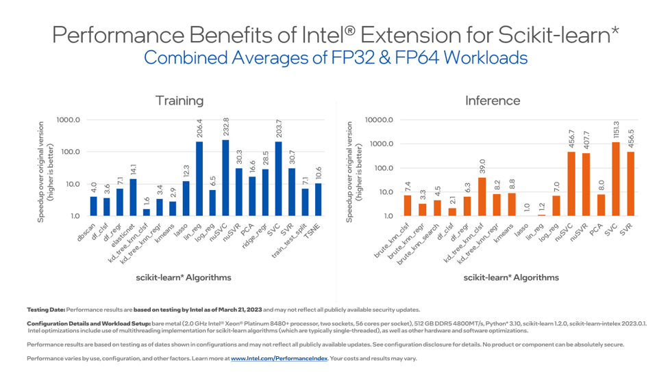
英特尔宣称 对SVC的加速可以达到203.7%，然而我们并没有看到这样的结果。 我们使用假设检验来看看英特尔的sklearn是不是显著地块？这里由于结果是相关的，而且不能假设是正态分布，所以使用 wilcoxon signed rank 检验。

from scipy.stats import wilcoxon

original_sklearn_time = [t.best for t in original_sklearn]
intel_sklearn_time = [t.best for t in intel_sklearn]
res_less = wilcoxon(intel_sklearn_time, original_sklearn_time, zero_method='zsplit',alternative='less' # 实验备则假设， intel_sklearn 用时更短
                    )
if res_less.pvalue > 0.05:
    print("Null hypothesis cannot be rejected, so I have to accept that intel_sklearn is not faster than original_sklearn. ")
res_less
res_greater = wilcoxon(intel_sklearn_time, original_sklearn_time, zero_method='zsplit', alternative='greater' # 实验备则假设，intel_sklearn 用时更长
                    )
res_less, res_greater

Sun 2024-11-17 01:36:45.594639

INFO     Null hypothesis cannot be rejected, so I have to accept that intel_sklearn is not faster     nucleus.py:53
         than original_sklearn.                                                                                    

(WilcoxonResult(statistic=7.0, pvalue=0.8125), WilcoxonResult(statistic=7.0, pvalue=0.3125))

可以看出，不能显著地说哪个更快，都是在随机误差范围之内。可以认为这两个方法一样快。

1.1.5.2 GPU上对SVM的加速

pip install thundersvm

from thundersvm import SVC

# thunder_svc = SVC(kernel='rbf', probability=True)
thunder_svc = SVC(gpu_id=2)
thunder_svc.fit(X_train, y_train)

在当前单元格或上一个单元格中执行代码时 Kernel 崩溃。

请查看单元格中的代码，以确定故障的可能原因。

单击<a href='https://aka.ms/vscodeJupyterKernelCrash'>此处</a>了解详细信息。

有关更多详细信息，请查看 Jupyter <a href='command:jupyter.viewOutput'>log</a>。

import pandas as pd

y_pred = thunder_svc.predict(X_test)
y_pred_proba = thunder_svc.predict_proba(X_test)
thunder_svc_res = compute_classification_metrics(y_test, y_pred_proba, logits_to_prob=False, y_pred=y_pred, labels=list(range(10)))
# thunder_svc_res, svc_res
res = []
for k, v in thunder_svc_res.items():
    delta = v - svc_res[k]
    # print(f"{k}: {v:.4f} ({delta:+.4f})")
    res.append(dict(metric=k, value=v, delta=delta))
pd.DataFrame(res)

	metric	value	delta
0	acc1	0.972222	0.000000
1	acc2	0.988889	0.005556
2	acc3	0.991667	0.002778
3	acc5	0.994444	0.002778
4	acc10	1.000000	0.000000
5	acc20	1.000000	0.000000
6	matthews_corrcoef	0.969250	0.000000
7	f1	0.972030	0.000000
8	precision	0.973182	0.000000
9	recall	0.971984	0.000000
10	balanced_accuracy	0.971984	0.000000
11	cohen_kappa	0.969134	0.000000
12	roc_auc	0.992732	-0.006617
13	hinge_loss	0.124893	0.005310
14	log_loss	0.370853	0.242670
15	acc1_pred	0.972222	0.000000

看来精度上和sklearn的SVC基本一致，基本没有差别，除了log_loss多一点。

thunder_svc_time = %timeit -o thunder_svc.fit(X_train, y_train)

164 ms ± 59.1 ms per loop (mean ± std. dev. of 7 runs, 1 loop each)

svc_time = %timeit -o svc.fit(X_train, y_train)

186 ms ± 4.74 ms per loop (mean ± std. dev. of 7 runs, 10 loops each)

这里时间是不相关的，所以使用 mannwhitneyu 检验。

from scipy.stats import mannwhitneyu

res_less = mannwhitneyu(thunder_svc_time.all_runs, svc_time.all_runs, alternative='less' # 实验备则假设， intel_sklearn mannwhitneyu
                    )
if res_less.pvalue > 0.05:
    print("We cannot reject the null hypothesis! ")
else:
    print("Null hypothesis rejected! ThunderSVC is significantly faster than SVC.")
res_less

Fri 2024-11-15 23:22:46.455835

INFO     Null hypothesis rejected! ThunderSVC is significantly faster than SVC.                         utils.py:77

MannwhitneyuResult(statistic=0.0, pvalue=0.0002913752913752914)

看来thundersvm在GPU上加速还是显著地更快一些。

1.2 实现 Hinge Loss+SGD 版本的 Soft Margin Linear SVM 并对其进行调参优化

现在我们已经调研并且运行了已有SVM库的代码，了解了他们的用法以及在MNIST数据集上的表现。接下来我们将手写实现SVM，以及对其进行优化。

接下来的内容请见文件 02svm_handy_crafted_linear。

本次Project的目录请见绪论 00svm。